Monopsony

In economics, a monopsony (from Ancient Greek μόνος (mónos) "single" + ὀψωνία (opsōnía) "purchase") is a market structure in which only one buyer interacts with many would-be sellers of a particular product. In microeconomic theory of monopsony, a single entity is assumed to have market power over terms of offer to its sellers, as the only purchaser of a good or service, much in the same manner that a monopolist can influence the price for its buyers in a monopoly, in which only one seller faces many buyers.

In addition to its use in microeconomic theory, monopsony and monopsonist are descriptive terms often used to describe a market where a single buyer substantially controls the market as the major purchaser of goods and services.

Etymology

The term was first introduced by Joan Robinson in her influential^[1] book, The Economics of Imperfect Competition, published in 1933. Robinson credited classics scholar Bertrand Hallward at the University of Cambridge with coining the term.^[2]

Overview

The term "monopsony power", in a manner similar to "monopoly power", is used by economists as a shorthand reference to buyers who face an upwardly sloping supply curve but that are not the only consumer; alternative terms are oligopsony or monopsonistic competition.

Static monopsony in a labor market

A monopsonist employer maximizes profits by choosing the employment level L, that equates the marginal revenue product (MRP) to the marginal cost MC, at point A. The wage is then determined on the supply curve, at point M, and is equal to w. By contrast, a competitive labor market would reach equilibrium at point C, where supply S equals demand. This would lead to employment L' and wage w'.

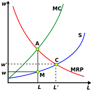
The standard, textbook monopsony model refers to static, partial equilibrium in a labor market with just one employer who pays the same wage to all the workers. The employer faces an upward-sloping labor supply curve (as generally contrasted with an infinitely elastic labor supply curve), represented by the S blue curve in the diagram on the right. This curve relates the wage paid, $w$ , to the level of employment, $L$ , and is denoted as an increasing function $w(L)$ . Total labor costs are given by $w(L)\cdot L$ . The firm has a total revenue $R$ , which increases with $L$ . The firm wants to choose $L$ to maximize profits, $P$ , which are given by:

P(L)=R(L)-w(L)\cdot L\,\!

At the maximum profit $P'(L)=0$ , so first-order condition for maximization is

0=R'(L)-w'(L)\cdot L-w(L)

where here $w'(L)$ is the derivative of the function $w(L),$ implying

R'(L)=w'(L)\cdot L+w(L).

The left-hand side of this expression, $R'(L)$ , is the marginal revenue product of labor (roughly, the extra revenue produced by an extra worker) and is represented by the red MRP curve in the diagram. The right-hand side is the marginal cost of labor (roughly, the extra cost due to an extra worker) and is represented by the green MC curve in the diagram. Notably, the marginal cost is higher than the wage $w(L)$ paid to the new worker by the amount

w'(L)L\,\!

This is because the firm has to increase the wage paid to all the workers it already employs whenever it hires an extra worker. In the diagram, this leads to an MC curve that is above the labor supply curve S.

The first-order condition for maximum profit is then satisfied at point A of the diagram, where the MC and MRP curves intersect. This determines the profit-maximising employment as L on the horizontal axis. The corresponding wage w is then obtained from the supply curve, through point M.

The monopsonistic equilibrium at M can be contrasted with the equilibrium that would obtain under competitive conditions. Suppose a competitor employer entered the market and offered a wage higher than that at M. Then every employee of the first employer would choose instead to work for the competitor. Moreover, the competitor would gain all the former profits of the first employer, minus a less-than-offsetting amount from the wage increase of the first employer's employees, plus profits arising from additional employees who decided to work in the market because of the wage increase. But the first employer would respond by offering an even higher wage, poaching the new rival's employees, and so forth. As a result, a group of perfectly competitive firms would be forced, through competition, to intersection C rather than M. Just as a monopoly is thwarted by the competition to win sales, minimizing prices and maximizing output, competition for employees between the employers in this case would maximize both wages and employment.

Welfare implications

The grey rectangle is a measure of the amount of economic welfare transferred from the workers to their employer(s) by monopsony power. The yellow triangle shows the overall deadweight loss inflicted on both groups by the monopsonistic restriction of employment. It is thus a measure of the market failure caused by monopsony.

The lower employment and wages caused by monopsony power have two distinct effects on the economic welfare of the people involved. First, it redistributes welfare away from workers and to their employer(s). Secondly, it reduces the aggregate (or social) welfare enjoyed by both groups taken together, as the employers' net gain is smaller than the loss inflicted on workers.

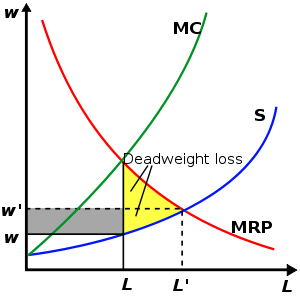
The diagram on the right illustrates both effects, using the standard approach based on the notion of economic surplus. According to this notion, the workers' economic surplus (or net gain from the exchange) is given by the area between the S curve and the horizontal line corresponding to the wage, up to the employment level. Similarly, the employers' surplus is the area between the horizontal line corresponding to the wage and the MRP curve, up to the employment level. The social surplus is then the sum of these two areas.

Following such definitions, the grey rectangle, in the diagram, is the part of the competitive social surplus that has been redistributed from the workers to their employer(s) under monopsony. By contrast, the yellow triangle is the part of the competitive social surplus that has been lost by both parties, as a result of the monopsonistic restriction of employment. This is a net social loss and is called deadweight loss. It is a measure of the market failure caused by monopsony power, through a wasteful misallocation of resources.

As the diagram suggests, the size of both effects increases with the difference between the marginal revenue product MRP and the market wage determined on the supply curve S. This difference corresponds to the vertical side of the yellow triangle, and can be expressed as a proportion of the market wage, according to the formula:

e={\frac {R'(w)-w}{w}}\,\!

The ratio $e$ has been called the rate of exploitation, and it can be easily shown that it equals the reciprocal of the elasticity of the labour supply curve faced by the firm. Thus the rate of exploitation is zero under competitive conditions, when this elasticity tends to infinity. Empirical estimates of $e$ by various means are a common feature of the applied literature devoted to the measurement of observed monopsony power.

Finally, it is important to notice that, while the gray-area redistribution effect could be reversed by fiscal policy (i.e., taxing employers and transferring the tax revenue to the workers), this is not so for the yellow-area deadweight loss. The market failure can only be addressed in one of two ways: either by breaking up the monopsony through anti-trust intervention, or by regulating the wage policy of firms. The most common kind of regulation is a binding minimum wage higher than the monopsonistic wage.

Minimum wage

With a binding minimum wage of w'' the marginal cost to the firm becomes the horizontal black MC' line, and the firm maximises profits at A with a higher employment L''. However, in this example, the minimum wage is higher than the competitive one, leading to involuntary unemployment equal to the segment AB.

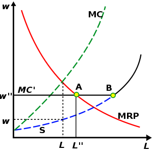
A binding minimum wage can be introduced either by law or through collective bargaining, and its possible effects in a special case are shown in the diagram on the right.

Here the minimum wage is w'', higher than the monopsonistic w. At this given wage the firm can now hire all the workers it wants, up to the supply curve, so that in the relevant employment range its marginal cost of labor becomes effectively constant and equal to w'',, as shown by the new black horizontal line MC'. Hence the firm maximizes profits at the new intersection point A, choosing the employment level L'', which is higher than the monopsonistic level L. As the reader can check, the rate of exploitation has been reduced to zero.

More generally, a binding minimum wage modifies the form of the supply curve faced by the firm, which becomes:

w={\begin{cases}w_{min},&{\mbox{if }}w_{min}\geq \;w(L)\\w(L),&{\mbox{if }}w_{min}\leq \;w(L)\end{cases}}\,\!

where $w(L)$ is the original supply curve and $w_{min}$ is the minimum wage. The new curve has thus a horizontal first branch and a kink at the point

w(L)=w_{min}\,\!

as is shown in the diagram by the kinked black curve MC' S. The resulting equilibria (the profit-maximizing choices that rational companies will make) can then fall into one of three classes according to the value taken by the minimum wage, as shown by the following table:

Profit Maximizing Choice In A Monopsonistic Labor Market Depends Upon The Minimum Wage Level
	Minimum Wage	Resulting Equilibrium
First Case	< than monopsony wage	unchanged from monopsony
Second Case	> monopsony wage but <= than competitive wage	at kink of supply curve
Third Case	> competitive wage	at intersection where minimum wage equals MRP

As it is now seen, the example illustrated by the diagram belongs to the third regime. As a result, there is an excess supply of labor – i.e. involuntary unemployment – equal to the segment AB. So, although the exploitation rate has vanished, there is still a deadweight loss to society. This illustrates the problems that may arise when the proper level of the binding minimum wage is not exactly known, or cannot be enforced for political reasons.

Yet, even when it is sub-optimal, a minimum wage higher than the market rate raises the level of employment anyway. This is a highly remarkable result, because it only follows under monopsony. Indeed, under competitive conditions any minimum wage higher than the market rate would actually reduce employment, according to classical economic models. Thus, spotting the effects on employment of newly introduced minimum wage regulations is among the indirect ways economists use to pin down monopsony power in selected labor markets.

To summarize: to the degree to which market conditions are monopsonistic, a minimum wage will not increase unemployment but decrease it. This has been demonstrated empirically in the study "Minimum Wages and Employment: A Case Study of the Fast Food Industry in New Jersey and Pennsylvania".^[3]

Wage discrimination

Just like a monopolist, a monopsonistic employer may find that its profits are maximized if it discriminates prices. In this case this means paying different wages to different groups of workers even if their MRP is the same, with lower wages paid to the workers who have a lower elasticity of supply of their labor to the firm.

Researchers have used this fact to explain at least part of the observed wage differentials whereby women often earn less than men, even after controlling for observed productivity differentials. Robinson's original application of monopsony (1938) was developed to explain wage differentials between equally productive women and men.^[4] Ransom and Oaxaca (2004) found that women's wage elasticity is lower than that of men for employees at a grocery store chain in Missouri, controlling for other factors typically associated with wage determination.^[5] Ransom and Lambson (2011) found that female teachers are paid less than male teachers due to differences in labor market mobility constraints facing women and men.^[6]

Some authors have argued informally that, while this is so for market supply, the reverse may somehow be true of the supply to individual firms. In particular, Manning and others have shown that, in the case of the UK Equal Pay Act, implementation has led to higher employment of women. Since the Act was effectively minimum wage legislation for women, this might perhaps be interpreted as a symptom of monopsonistic discrimination.

Empirical problems

Sources of labour monopsony power

The simpler explanation of monopsony power in labour markets is barriers to entry on the demand side. In all such cases, oligopsony would result from oligopoly in the product markets of the industries that use that type of labour as input. If the hypothesis was generally true, one would then find a positive statistical correlation between exploitation, on one side, and industry concentration and firm size on the other. However, numerous statistical studies document significant positive correlations between firm or establishment size and wages. These results, by themselves inconsistent with the oligopoly-oligopsony hypothesis, may be due to the prevalence of other factors, such as efficiency wages.

However, monopsony power might also be due to circumstances affecting entry of workers on the supply side, directly reducing the elasticity of labour supply to firms. Paramount among these are moving costs for workers, which are also a cause of differentiation among potential employees, possibly leading to discrimination (see above). But a similar effect might also be produced by all the institutional factors that limit labour mobility between firms, including job protection legislation. The vetting of employees in the government or the defense sector is another source of monopsonistic competition, as are requirements for professional certification, for example, a medical degree. Finally, as already noticed, a significant reduction in the short-run elasticity of supply may come from information costs and search behaviour.

An alternative that has been suggested as a source of monopsony power is worker preferences over job characteristics (Bhaskar and To, 1999; Bhaskar, Manning and To, 2002). Such job characteristics can include distance from work, type of work, location, the social environment at work, etc. If different workers have different preferences, employers have local monopsony power over workers that strongly prefer working for them.

Finally, monopsony power will occur when the average revenue product of labor increases with the amount of labor employed, due to economies of scale. In this case, the perfectly competitive solution (workers are paid their marginal revenue product) is not stable. In the long run, the firm may set wages equal to the average revenue product of labor, or engage in wage discrimination, paying wages closer to marginal product to markets (or workers) with higher elasticity of supply.

References

↑ Kerr, Prue; Harcourt, Geoff (2002). Joan Robinson: Critical Assessments of Leading Economists. Taylor & Francis. pp. 2–3. ISBN 0-415-21743-1
↑ Thornton, Rupert J. (2004). "Retrospectives: How Joan Robinson and B. L. Hallward Named Monopsony". Journal of Economic Perspectives. 18 (2): 257–261. doi:10.1257/0895330041371240.
↑ http://www.nber.org/papers/w4509
↑ http://www.u.arizona.edu/~rlo/696i/Monopsony_Model_Latex.pdf
↑ http://dataspace.princeton.edu/jspui/bitstream/88435/dsp01nk322d34x/1/540.pdf
↑ "Monopsony, mobility, and sex differences in pay : Missouri school teachers". econbiz.de.

External links

"Monopsony in American Labor Markets". EH.NET's Encyclopedia.

Microeconomics

Major topics	Aggregation Bilateral monopoly Budget Consumer Convexity and non-convexity Cost Cost–benefit analysis Deadweight loss Distribution Duopoly Economies of scale Economies of scope Elasticity Equilibria Exchange Expected utility Externality Firms General equilibrium Household Income–consumption curve Information Indifference curve Intertemporal choice Marginal cost Market failure Market structure Monopoly Monopsony Oligopoly Preferences Production Profit Public goods Returns to scale Risk aversion Scarcity Shortage Social choice Sunk costs Supply & demand Surplus Uncertainty Utility Welfare

Subfields	Behavioral Business Computational Statistical decision theory Econometrics Experimental Game theory Industrial organization Labor Managerial Mathematical economics Microfoundations of macroeconomics Operations research Optimization

This article is issued from Wikipedia - version of the 11/3/2016. The text is available under the Creative Commons Attribution/Share Alike but additional terms may apply for the media files.