Income–consumption curve

Economics
Phillips curve graph, illustrating an economic principle
Index Outline Category
History Types Classification
History of economics Economic history (academic study) Schools of economics Microeconomics Macroeconomics Methodology Heterodox economics JEL classification codes
Concepts Theory Techniques
Econometrics Economic growth Economic system Experimental economics Mathematical economics Game theory Market National accounting
By application
Agricultural Behavioral Business Computational Cultural Demographic Development Digitization Ecological Education Environmental Evolutionary Expeditionary Geography Health Industrial organization Information International Knowledge Labour Law Managerial Monetary / Financial Natural resource Personnel Public / Welfare economics Regional Rural Service Urban Welfare
Lists
Economists Publications (journals)
Business and economics portal

In economics and particularly in consumer choice theory, the income-consumption curve is a curve in a graph in which the quantities of two goods are plotted on the two axes; the curve is the locus of points showing the consumption bundles chosen at each of various levels of income.

The income effect in economics can be defined as the change in consumption resulting from a change in real income.^[1] This income change can come from one of two sources: from external sources, or from income being freed up (or soaked up) by a decrease (or increase) in the price of a good that money is being spent on. The effect of the former type of change in available income is depicted by the income-consumption curve discussed in the remainder of this article, while the effect of the freeing-up of existing income by a price drop is discussed along with its companion effect, the substitution effect, in the article on the latter.

The consumer's preferences, monetary income and prices play an important role in solving the consumer's optimization problem (choosing how much of various goods to consume so as to maximize their utility subject to a budget constraint). The comparative statics of consumer behavior investigates the effects of changes in the exogenous or independent variables (especially prices and money incomes of the consumers) on the chosen values of the endogenous or dependent variables (the consumer's demands for the goods). When the income of the consumer rises with the prices held constant, the optimal bundle chosen by the consumer changes as the feasible set available to him changes. The income–consumption curve is the set of tangency points of indifference curves with the various budget constraint lines, with prices held constant, as income increases shifting the budget constraint out.

Consumer theory

Figure 1: An increase in the income, with the prices of all goods fixed, causes consumers to alter their choice of market basket. The extreme left and right indifference curves belong to different individuals with different preferences, while the three central indifference curves belong to one individual for whom the income-consumption curve is shown.

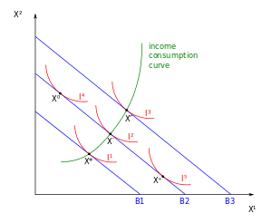
The income effect is a phenomenon observed through changes in purchasing power. It reveals the change in quantity demanded brought by a change in real income. The figure 1 on the left shows the consumption patterns of the consumer of two goods X¹ and X², the prices of which are p₁ and p₂ respectively. The initial bundle X^*, is the bundle which is chosen by the consumer on the budget line B₁. An increase in the money income of the consumer, with p₁ and p₂ constant, will shift the budget line outward parallel to itself.

In the figure, this means that the change in the money income of the consumer will shift the budget line B1 outward parallel to itself to B2 where the bundle X^' bundle will be chosen. Again, an increase in the money income of the consumer will push the budget line B2 outward parallel to itself to B3 where the bundle X^" will be the bundle which will be chosen. Thus, it can be said that, with variations in income of the consumers and with the prices held constant the income–consumption curve can be traced out as the set of optimal points.

Income–consumption curve for different goods

In the case illustrated with the help of Figure 1 both X¹ and X² are normal goods in which case, the demand for the good increases as money income rises. However, if the consumer has different preferences, he has the option to choose X⁰ or X⁺ on budget line B2. As the income of the consumer rises,and the consumer chooses X⁰ instead of X^' i.e. if the consumer's indifference curve is I⁴ and not I², then the demand for X¹ would fall . In that case, X¹ would be called an inferior good i.e. demand for good X¹ decreases with a rise in income of the consumer. Thus, a rise in income of the consumer may lead his demand for a good to rise, fall or not change at all. It is important to note here that, the knowledge of preferences of the consumer is essential to predict whether a particular good is inferior or normal.

Normal goods

Figure 2: Income-consumption curve for Normal goods

In the figure 2 to the left, B1, B2 and B3 are the different budget lines and I¹, I² and I³ are the indifference curves that are available to the consumer. As shown earlier, as the income of the consumer rises, the budget line moves outwards parallel to itself. In this case, from initial bundle X^*, with an increase in the income of the consumer the budget line moves from B1 to B2 and the consumer would choose X^' bundle and subsequently, with a further rise in consumer's income the budget line moves from B2 to B3 and the consumer would choose X^" bundle and so on. The consumer would thus maximize his utility at the points X^*, X^' and X^", and by joining these points, the income-consumption curve can be obtained.^[2]

The upward sloping income-consumption curve implies that there will be an increase in the demand for both X¹ and X² as the income of the consumer rises and will cause the demand curves of the goods to shift to the right.^[3] When the income-consumption curve has a positive slope then the income elasticity of demand will be positive. The greater the shifts of the demand curve to the right, the greater the income-elasticity of demand. In such a case, the goods will be normal goods.^[3]

Inferior goods

Figure 3: with an increase in the income of demand for normal good X² rises while, demand for inferior good X¹ falls.

The figure on the right (figure 3), shows the consumption patterns of the consumer of two goods X¹ and X², the prices of which are p₁ and p₂ respectively, where B1 and B2 are the budget lines and I¹ and I² are the indifference curves. Figure 3 clearly shows that, with a rise in the income of the consumer, the initial budget line B1 moves outward parallel to itself to B2 and the consumer now chooses X^' bundle to the initial bundle X^*. The figure shows that, the demand for X² has risen from X²₁ to X²₂ with an outward shift of the budget line from B1 to B2 (caused due to rise in the income of the consumer). This essentially means that, good X² is a normal good as the demand for X² rose with an increase in the income of the consumer.

In contrast, it is to be noted from the figure, that the demand for X¹ has fallen from X¹₁ to X¹₂ with an outward shift of the budget line from B1 to B2 (caused due to rise in the income of the consumer). This implies that, good X¹ is an inferior good as the demand for X¹ fell with an increase in the income of the consumer.

The consumer maximizes his utility at points X^* and X^' and by joining these points, the income–consumption curve can be obtained.^[2] In figure 3, the income–consumption curve bends back on itself as with an increase income, the consumer demands more of X² and less of X¹.^[4] The income–consumption curve in this case is negatively sloped and the income elasticity of demand will be negative.^[3] Also the price effect for X² is positive, while it is negative for X¹.^[4]

$\Delta X_{n}^{1}$ is the change in the demand for good 1 when we change income from $m'$ to $m$ , holding the price of good 1 fixed at $p_{1}$ :

$\Delta X_{n}^{1}=X^{1}(p_{1},m)-X^{1}(p_{1},m').$

Perfect substitutes

Figure4: Income–consumption curve for perfect substitutes

The figure on the right depicts the case of two goods X¹ and X² which are perfect substitutes, prices of which are p₁ and p₂ respectively. Here, I¹, I², I³, I⁴ and I⁵ are the straight line indifference curves, B1, B2 and B3 are the budget constraints and X^*, X^' and X^" are the bundles chosen by the consumer. If it is assumed that p₁ < p₂ then the consumer would consume only X¹ as this would maximize his utility.^[5]

In the figure on the right, B1 is the initial budget line and the consumer chooses X^* as his optimal bundle and as the money income of the consumer rises, his budget line will shift outward and parallel to itself to B2. At the budget line B2 and the indifference curve I⁴, the consumer will choose X^'. Subsequently, as the income rises further, the budget line will again shift outward and parallel to itself to B3, where, the consumer will choose the optimal bundle X^".

Thus, it can be said that, the amount of good X¹ that the consumer consumes will increase, with an increase in the income of the consumer.^[6] Thus, the income–consumption curve for the perfect substitutes X¹ and X² will be the horizontal axis.^[5]

Perfect complements

Figure 5: Income–consumption curve for perfect complements

In case of perfect complements, the same amount of goods will be consumed by the consumer irrespective of say income, prices etc.^[6] As the level of consumption remains the same, the income–consumption curve for perfect complements is the diagonal line passing through the origin as shown in Figure 5 on the left.

In the figure on the left, X^*, X^' and X^" are the utility maximization points where the budget constraint lines B1, B2 and B3 touch the kinks of the L-shaped indifference curves I¹, I² and I³ respectively.^[5] By joining these points of utility maximization, the income–consumption curve for perfect complements is obtained.

Cobb–Douglas preferences

The demand functions for both good 1 with quantity demanded X₁ and good 2 with quantity demanded X₂ under Cobb-Douglas preferences are linear functions of income m, and thus the income-consumption curve will be a straight line through the origin.^[6] If

u(X_{1},X_{2})=X_{1}^{a}X_{2}^{{(1-a)}}\,

then the demand for good 1 will have the form $X_{1}=am/p_{1}.$ ^[6]

If p₁ is kept at a fixed value, then this will be a linear function of m. By doubling m, the demand will double. In fact, if m is multiplied by any positive number, say t, the demand will be multiplied with the same amount.

For good 2, the demand is given by $X_{2}=(1-a)m/p_{2}\,$ .^[6] This too is clearly linear and homogeneous in m, thus making the income-consumption curves for both the goods 1 and 2 straight lines passing through the origin.

Income–consumption curve and Engel curves

Main article: Engel curve

At each level of income level, say m, there would be an optimal choice for each of the goods. If only the case of a good say, good X¹ is taken, the optimal choice at each set of prices and income or in other words, the demand function for good X¹ can be written as:

$X^{1}=X^{1}(p_{1},p_{2},m)\,$ ^[6]

Here, p₁ is the price of good X¹, p₂ is the price of good X² and m is the income of the consumer.

If the prices of the goods X¹ and X² are held constant and the changes in demand are observed in relation to changes in income, the Engel curve can be generated. With all prices held constant, the Engel curve can be defined as a graph depicting the demand for one good as a function of income.^[6]

References

↑ Sullivan, Arthur; Sheffrin, Steven M. (2003). Economics: Principles in Action. Upper Saddle River: Pearson Prentice Hall. p. 80. ISBN 0-13-063085-3.
1 2 "Archived copy" (PDF). Archived from the original on October 20, 2012. Retrieved September 11, 2011. CS1 maint: Unfit url (link)
1 2 3 Rubinfeld, Daniel; Pindyck, Robert (1995). Microeconomics. Mainland China: Tsinghua University Press/Prentice-Hall. p. 699. ISBN 7-302-02494-4.
1 2 http://economicsconcepts.com/application_of_indifference_curves.htm
1 2 3
1 2 3 4 5 6 7 R Varian, Hal (2006). Intermediate Microeconomics : A modern approach. W.W. Norton & Co. p. 754. ISBN 0-393-92702-4.

Microeconomics

Major topics	Aggregation Bilateral monopoly Budget Consumer Convexity and non-convexity Cost Cost–benefit analysis Deadweight loss Distribution Duopoly Economies of scale Economies of scope Elasticity Equilibria Exchange Expected utility Externality Firms General equilibrium Household Income–consumption curve Information Indifference curve Intertemporal choice Marginal cost Market failure Market structure Monopoly Monopsony Oligopoly Preferences Production Profit Public goods Returns to scale Risk aversion Scarcity Shortage Social choice Sunk costs Supply & demand Surplus Uncertainty Utility Welfare

Subfields	Behavioral Business Computational Statistical decision theory Econometrics Experimental Game theory Industrial organization Labor Managerial Mathematical economics Microfoundations of macroeconomics Operations research Optimization

This article is issued from Wikipedia - version of the 11/3/2016. The text is available under the Creative Commons Attribution/Share Alike but additional terms may apply for the media files.