IBM alignment models

IBM alignment models are a sequence of increasingly complex models used in statistical machine translation to train a translation model and an alignment model, starting with lexical translation probabilities and moving to reordering and word duplication.^[1] They have underpinned the majority of statistical machine translation systems for almost twenty years. These models offer principled probabilistic formulation and (mostly) tractable inference.^[2]

The original work on statistical machine translation at IBM proposed five models, and a model 6 was proposed later. The sequence of the six models can be summarized as:

Model 1: lexical translation
Model 2: additional absolute alignment model
Model 3: extra fertility model
Model 4: added relative alignment model
Model 5: fixed deficiency problem.
Model 6: Model 4 combined with a HMM alignment model in a log linear way

Model 1

IBM Model 1 is weak in terms of conducting reordering or adding and dropping words. In most cases, words that follow each other in one language would have a different order after translation, but IBM Model 1 treats all kinds of reordering as equally possible.

Another problem while aligning is the fertility (the notion that input words would produce a specific number of output words after translation). In most cases one input word will be translated into one single word, but some words will produce multiple words or even get dropped (produce no words at all). The fertility of word models addresses this aspect of translation. While adding additional components increases the complexity of models, the main principles of IBM Model 1 are constant.^[3]

Model 2

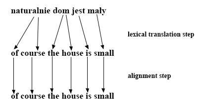
The IBM Model 2 has an additional model for alignment that is not present in Model 1. For example, using only IBM Model 1 the translation probabilities for these translations would be the same:

The IBM Model 2 addressed this issue by modeling the translation of a foreign input word in position i to a native language word in position j using an alignment probability distribution defined as:

a(i\lor j,l_{e},l_{f})

In the above equation, the length of the input sentence f is denoted as l_f, and the length of the translated sentence e as l_e. The translation done by IBM Model 2 can be presented as a process divided into two steps (lexical translation and alignment).

Assuming $t(e\mid f)$ is the translation probability and $a(i\lor j,l_{e},l_{f})$ is the alignment probability, IBM Model 2 can be defined as:

p(e,a\mid f)=\in \prod _{j=1}^{l_{e}}t(e_{j}\lor f_{a\mid j})a(a(j)\lor j,l_{e},l_{f})

In this equation, the alignment function $a$ maps each output word $j$ to a foreign input position $a(j)$ .^[4]

Model 3

The fertility problem is addressed in IBM Model 3. The fertility is modeled using probability distribution defined as:

n(\phi \lor f)

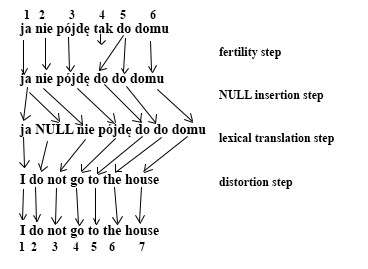
For each foreign word $j$ , such distribution indicates to how many output words $\phi$ it usually translates. This model deals with dropping input words because it allows $\phi =0$ . But there is still an issue when adding words. For example, the English word do is often inserted when negating. This issue generates a special NULL token that can also have its fertility modeled using a conditional distribution defined as:

n(\varnothing \lor NULL)

The number of inserted words depends on sentence length. This is why the NULL token insertion is modeled as an additional step: the fertility step. It increases the IBM Model 3 translation process to four steps:

The last step is called distortion instead of alignment because it is possible to produce the same translation with the same alignment in different ways.^[5]

IBM Model 3 can be mathematically expressed as:

P(S\mid E,A)=\prod _{i=1}^{I}\Phi _{i}!n(\Phi \mid e_{j})*\prod _{j=1}^{J}t(f_{j}\mid e_{a_{j}})*\prod _{j:a(j)\neq 0}^{J}d(j\mid a_{j},I,J)*({\begin{array}{c}J-\Phi _{0}\\\Phi _{0}\end{array}})p_{0}^{\Phi _{0}}p_{1}^{J}

where $\Phi _{i}$ represents the fertility of $e_{i}$ , each source word $s$ is assigned a fertility distribution $n$ , and $I$ and $J$ refer to the absolute lengths of the target and source sentences, respectively.^[6]

Model 4

In IBM Model 4, each word is dependent on the previously aligned word and on the word classes of the surrounding words. Some words tend to get reordered during translation more than others (e.g. adjective–noun inversion when translating Polish to English). Adjectives often get moved before the noun that precedes them. The word classes introduced in Model 4 solve this problem by conditioning the probability distributions of these classes. The result of such distribution is a lexicalized model. Such a distribution can be defined as follows:

For the initial word in the cept: $d_{1}(j-\odot _{[i-1]}\lor A(f_{[i-1]}),B(e_{j}))$

For additional words: $d_{1}(j-\pi _{i,k-1}\lor B(e_{j}))$

where $A(f)$ and $B(e)$ functions map words to their word classes, and $e_{j}$ and $f_{[i-1]}$ are distortion probability distributions of the words. The cept is formed by aligning each input word $f_{i}$ to at least one output word.^[7]

Both Model 3 and Model 4 ignore if an input position was chosen and if the probability mass was reserved for the input positions outside the sentence boundaries. It is the reason for the probabilities of all correct alignments not sum up to unity in these two models (deficient models).^[7]

Model 5

IBM Model 5 reformulates IBM Model 4 by enhancing the alignment model with more training parameters in order to overcome the model deficiency.^[8] During the translation in Model 3 and Model 4 there are no heuristics that would prohibit the placement of an output word in a position already taken. In Model 5 it is important to place words only in free positions. It is done by tracking the number of free positions and allowing placement only in such positions. The distortion model is similar to IBM Model 4, but it is based on free positions. If $v_{j}$ denotes the number of free positions in the output, the IBM Model 5 distortion probabilities would be defined as:^[9]

For the initial word in the cept: $d_{1}(v_{j}\lor B(e_{j}),v_{\odot i-1},v_{max})$

For additional words: $d_{1}(v_{j}-v_{\pi _{i,k-1}}\lor B(e_{j}),v_{max'})$

The alignment models that use first-order dependencies like the HMM or IBM Models 4 and 5 produce better results than the other alignment methods. The main idea of HMM is to predict the distance between subsequent source language positions. On the other hand, IBM Model 4 tries to predict the distance between subsequent target language positions. Since it was expected to achieve better alignment quality when using both types of such dependencies, HMM and Model 4 were combined in a log-linear manner in Model 6 as follows:^[10]

p_{6}(f,a\lor e)={\frac {p_{4}(f,a\lor e)^{\alpha }*p_{HMM}(f,a\lor e)}{\sum _{a',f'}p_{4}(f',a'\lor e)^{\alpha }*p_{HMM}(f',a'\lor e)}}

where the interpolation parameter $\alpha$ is used in order to count the weight of Model 4 relatively to the hidden Markov model. A log-linear combination of several models can be defined as $p_{k}(f,a\mid e)$ with $k=1,2,\dotsc ,K$ as:

p_{6}(f,a\lor e)={\frac {\prod _{k=1}^{K}p_{k}(f,a\lor e)^{\alpha _{k}}}{\sum _{a',f'}\prod _{k=1}^{K}p_{k}(f',a'\mid e)^{\alpha _{k}}}}

The log-linear combination is used instead of linear combination because the $P_{r}(f,a\mid e)$ values are typically different in terms of their orders of magnitude for HMM and IBM Model 4.^[11]

References

↑ "IBM Models". SMT Research Survey Wiki. 11 September 2015. Retrieved 26 October 2015.
↑ Yarin Gal, Phil Blunsom (12 June 2013). "A Systematic Bayesian Treatment of the IBM Alignment Models" (PDF). University of Cambridge. Retrieved 26 October 2015.
↑ Wołk, K.; Marasek, K. "Real-Time Statistical Speech Translation". Advances in Intelligent Systems and Computing. Springer. 275: 107–114. ISBN 978-3-319-05950-1. ISSN 2194-5357.
↑ Och, Franz Josef; Ney, Hermann (2003). "A systematic comparison of various statistical alignment models". Computational linguistics (29): 19–51.
↑ Wołk K., Marasek K. (2014). Polish-English Speech Statistical Machine Translation Systems for the IWSLT 2014. Proceedings of the 11th International Workshop on Spoken Language Translation, Lake Tahoe, USA.
↑ FERNÁNDEZ, Pablo Malvar. Improving Word-to-word Alignments Using Morphological Information. 2008. PhD Thesis. San Diego State University.
1 2 Schoenemann, Thomas (2010). Computing optimal alignments for the IBM-3 translation model. Proceedings of the Fourteenth Conference on Computational Natural Language Learning. Association for Computational Linguistics. pp. 98–106.
↑ KNIGHT, Kevin. A statistical MT tutorial workbook. Manuscript prepared for the 1999 JHU Summer Workshop, 1999.
↑ Brown, Peter F. (1993). "The mathematics of statistical machine translation: Parameter estimation". Computational linguistics (19): 263–311.
↑ Vulić I. (2010). "Term Alignment. State of the Art Overview" (PDF). Katholieke Universiteit Leuven. Retrieved 26 October 2015.
↑ Wołk, K. (2015). "Noisy-Parallel and Comparable Corpora Filtering Methodology for the Extraction of Bi-Lingual Equivalent Data at Sentence Level". Computer Science (16.2): 169–184.

This article is issued from Wikipedia - version of the 11/14/2016. The text is available under the Creative Commons Attribution/Share Alike but additional terms may apply for the media files.