Forward volatility

Forward volatility is a measure of the implied volatility of a financial instrument over a period in the future, extracted from the term structure of volatility (which refers to how implied volatility differs for related financial instruments with different maturities).

Underlying principle

The variance is the square of differences of measurements from the mean divided by the number of samples. The standard deviation is the square root of the variance. The standard deviation of the continuously compounded returns of a financial instrument is called volatility.

The (yearly) volatility in a given asset price or rate over a term that starts from $t_0=0$ corresponds to the spot volatility for that underlying, for the specific term. A collection of such volatilities forms a volatility term structure, similar to the yield curve. Just as forward rates can be derived from a yield curve, forward volatilities can be derived from a given term structure of volatility.

Derivation

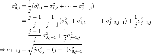
Given that the underlying random variables for non overlapping time intervals are independent, the variance is additive (see variance). So for yearly time slices we have the annualized volatility as

$\begin{align} \sigma_{0,j}^2 &= \frac{1}{j}(\sigma_{0,1}^2 + \sigma_{1,2}^2 + \cdots + \sigma_{j-2,j-1}^2 + \sigma_{j-1,j}^2)\\ \Rightarrow \sigma_{j-1,j} &=\sqrt{j\sigma_{0,j}^2-\sum_{k=1}^{j-1}\sigma_{k-1,k}^2}, \end{align}$

where

j=1,2,\ldots

is the number of years and the factor

\frac{1}{j}

scales the variance so it is a yearly one

\sigma_{i,\,j}

is the current (at time 0) forward volatility for the period

[i,\,j]

\sigma_{0,\,j}

the spot volatility for maturity

j

To ease computation and get a non-recursive representation, we can also express the forward volatility directly in terms of spot volatilities:^[1]

$\begin{align} \sigma_{0,j}^2 &= \frac{1}{j}(\sigma_{0,1}^2 + \sigma_{1,2}^2 + \cdots + \sigma_{j-1,j}^2)\\ &= \frac{j-1}{j}\cdot\frac{1}{j-1}(\sigma_{0,1}^2 + \sigma_{1,2}^2 + \cdots + \sigma_{j-2,j-1}^2) + \frac{1}{j}\sigma_{j-1,j}^2\\ &= \frac{j-1}{j}\,\sigma_{0,j-1}^2 + \frac{1}{j}\sigma_{j-1,j}^2 \\ \Rightarrow \sigma_{j-1,j} &=\sqrt{j\sigma_{0,j}^2-(j-1)\sigma_{0,j-1}^2} \end{align}$

Following the same line of argumentation we get in the general case with $t_0<t<T$ for the forward volatility seen at time $t_0$ :

$\sigma_{t,T}=\sqrt{\frac{(T-t_0)\sigma_{t_0,T}^2-(t-t_0)\sigma_{t_0,t}^2}{T-t}}$ ,

which simplifies in the case of $t_0=0$ to

$\sigma_{t,T}=\sqrt{\frac{T\sigma_{0,T}^2-t\sigma_{0,t}^2}{T-t}}$ .

Example

The volatilities in the market for 90 days are 18% and for 180 days 16.6%. In our notation we have $\sigma_{0,\,0.25}$ = 18% and $\sigma_{0,\,0.5}$ = 16.6% (treating a year as 360 days). We want to find the forward volatility for the period starting with day 91 and ending with day 180. Using the above formular and setting $t_0=0$ we get

$\sigma_{0.25,\,0.5}=\sqrt{\frac{0.5\cdot 0.166^2-0.25\cdot 0.18^2}{0.25}}=0.1507\approx 15.1\%$ .

References

↑ Taleb, Nassim Nicholas (1997). Dynamic Hedging: Managing Vanilla and Exotic Options. New York: John Wiley & Sons. ISBN 0-471-15280-3, pg 154

This article is issued from Wikipedia - version of the 10/28/2014. The text is available under the Creative Commons Attribution/Share Alike but additional terms may apply for the media files.