Cost–volume–profit analysis

Accounting

Historical cost Constant purchasing power Management Tax
Major types Auditing Cost Forensic Financial Fund Governmental Management Social Tax
Key concepts Accounting period Accrual Constant purchasing power Economic entity Fair value Going concern Historical cost Matching principle Materiality Revenue recognition Unit of account
Selected accounts Assets Cash Cost of goods sold Depreciation / Amortization Equity Expenses Goodwill Liabilities Profit Revenue
Accounting standards Generally-accepted principles Generally-accepted auditing standards Convergence International Financial Reporting Standards International Standards on Auditing Management Accounting Principles
Financial statements Annual report Balance sheet Cash-flow Equity Income Management discussion Notes to the financial statements
Bookkeeping Bank reconciliation Debits and credits Double-entry system FIFO and LIFO Journal Ledger / General ledger T accounts Trial balance
Auditing Financial Internal Firms Report
People and organizations Accountants Accounting organizations Luca Pacioli
Development History Research Positive accounting Sarbanes–Oxley Act
Business portal

Cost–volume–profit (CVP), in managerial economics, is a form of cost accounting. It is a simplified model, useful for elementary instruction and for short-run decisions.

Overview

A critical part of CVP analysis is the point where total revenues equal total costs (both fixed and variable costs). At this break-even point, a company will experience no income or loss. This break-even point can be an initial examination that precedes more detailed CVP analysis.

CVP analysis employs the same basic assumptions as in breakeven analysis. The assumptions underlying CVP analysis are:

The behavior of both costs and revenues are linear throughout the relevant range of activity. (This assumption precludes the concept of volume discounts on either purchased materials or sales.)
Costs can be classified accurately as either fixed or variable.
Changes in activity are the only factors that affect costs.
All units produced are sold (there is no ending finished goods inventory).
When a company sells more than one type of product, the product mix (the ratio of each product to total sales) will remain constant.

The components of CVP analysis are:

Level or volume of activity
Unit selling prices
Variable cost per unit
Total fixed costs

Assumptions

CVP assumes the following:

Constant sales price;
Constant variable cost per unit;
Constant total fixed cost;
Units sold equal units produced.

These are simplifying, largely linearizing assumptions, which are often implicitly assumed in elementary discussions of costs and profits. In more advanced treatments and practice, costs and revenue are nonlinear and the analysis is more complicated, but the intuition afforded by linear CVP remains basic and useful.

One of the main methods of calculating CVP is profit–volume ratio which is (contribution /sales)*100 = this gives us profit–volume ratio.

contribution stands for sales minus variable costs.

Therefore it gives us the profit added per unit of variable costs.

Model

Basic graph

The assumptions of the CVP model yield the following linear equations for total costs and total revenue (sales):

{\text{Total costs}}={\text{fixed costs}}+({\text{unit variable cost}}\times {\text{number of units}}

)

{\text{Total revenue}}={\text{sales price}}\times {\text{number of units}}

These are linear because of the assumptions of constant costs and prices, and there is no distinction between units produced and units sold, as these are assumed to be equal. Note that when such a chart is drawn, the linear CVP model is assumed, often implicitly.

In symbols:

{\text{TC}}={\text{TFC}}+{\text{V}}\times {\text{X}}

{\text{TR}}={\text{P}}\times {\text{X}}

where

TC = Total costs
TFC = Total fixed costs
V = Unit variable cost (variable cost per unit)
X = Number of units
TR = S = Total revenue = Sales
P = (Unit) sales price

Profit is computed as TR-TC; it is a profit if positive, a loss if negative.

Break down

Costs and sales can be broken down, which provide further insight into operations.

One can decompose total costs as fixed costs plus variable costs:

{\text{TC}}={\text{TFC}}+{\text{V}}\times {\text{X}}

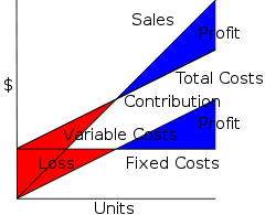
Following a matching principle of matching a portion of sales against variable costs, one can decompose sales as contribution plus variable costs, where contribution is "what's left after deducting variable costs". One can think of contribution as "the marginal contribution of a unit to the profit", or "contribution towards offsetting fixed costs".

In symbols:

{\begin{aligned}{\text{TR}}&={\text{P}}\times {\text{X}}\\&={\bigl (}\left({\text{P}}-{\text{V}}\right)+{\text{V}}{\bigr )}\times {\text{X}}\\&=\left({\text{C}}+{\text{V}}\right)\times {\text{X}}\\&={\text{C}}\times {\text{X}}+{\text{V}}\times {\text{X}}\end{aligned}}

where

C = Unit Contribution (Margin)

Subtracting variable costs from both costs and sales yields the simplified diagram and equation for profit and loss.

In symbols:

{\begin{aligned}{\text{PL}}&={\text{TR}}-{\text{TC}}\\&=\left({\text{C}}+{\text{V}}\right)\times {\text{X}}-\left({\text{TFC}}+{\text{V}}\times {\text{X}}\right)\\&={\text{C}}\times {\text{X}}-{\text{TFC}}\end{aligned}}

Diagram relating all quantities in CVP.

These diagrams can be related by a rather busy diagram, which demonstrates how if one subtracts variable costs, the sales and total costs lines shift down to become the contribution and fixed costs lines. Note that the profit and loss for any given number of unit sales is the same, and in particular the break-even point is the same, whether one computes by sales = total costs or as contribution = fixed costs. Mathematically, the contribution graph is obtained from the sales graph by a shear, to be precise $\left({\begin{smallmatrix}1&0\\-V&1\end{smallmatrix}}\right)$ , where V are unit variable costs.

Applications

CVP simplifies the computation of breakeven in break-even analysis, and more generally allows simple computation of target income sales. It simplifies analysis of short run trade-offs in operational decisions.

Limitations

CVP is a short run, marginal analysis: it assumes that unit variable costs and unit revenues are constant, which is appropriate for small deviations from current production and sales, and assumes a neat division between fixed costs and variable costs, though in the long run all costs are variable. For longer-term analysis that considers the entire life-cycle of a product, one therefore often prefers activity-based costing or throughput accounting.^[1]

When we analyze CVP is where we demonstrate the point at which in a firm there will be no profit nor loss means that firm works in breakeven situation

1. Segregation of total costs into its fixed and variable components is always a daunting task to do. 2. Fixed costs are unlikely to stay constant as output increases beyond a certain range of activity. 3. The analysis is restricted to the relevant range specified and beyond that the results can become unreliable. 4. Aside from volume, other elements like inflation, efficiency, capacity and technology impact on costs 5. Impractical to assume sales mix remain constant since this depends on the changing demand levels. 6. The assumption of linear property of total cost and total revenue relies on the assumption that unit variable cost and selling price are always constant. In real life it is valid within relevant range or period and likely to change.

Notes

↑ The Controversy over the contribution margin approach, in MAAW, Chapter 11.

Library resources about Cost-volume-profit analysis
Resources in your library

This article is issued from Wikipedia - version of the 11/23/2015. The text is available under the Creative Commons Attribution/Share Alike but additional terms may apply for the media files.

Cost–volume–profit analysis

Overview

Assumptions

Model

Basic graph

Break down

Applications

Limitations

See also

Notes